There is a dirty secret at the heart of the modern artificial intelligence data center: our most advanced silicon spends over ninety percent of its time doing absolutely nothing.
When an enterprise pays thousands of dollars an hour to lease an eight-way cluster of NVIDIA H100 or H200 SXM5 GPUs, they imagine those 16,000 Tensor Cores executing dense mathematical transformations at near-lightspeed. In reality, during single-stream autoregressive token generation, those Tensor Cores sit starved, idling between instruction cycles. The cluster is throttled not by compute capacity, but by the physical limits of moving bytes across high-bandwidth memory (HBM) buses.
For eight years—from the original Transformer architecture through GPT-4, Claude 3.5 Sonnet, and early reasoning systems—the generative AI industry accepted a crippling computational tax: sequential autoregression. Generating token $t+1$ strictly required the completed output of token $t$.
This sequential dependency forced high-performance computing back into the Von Neumann bottleneck.
The breakthrough that has rewritten inference economics in 2026 is Speculative Decoding—not as a speculative toy or an academic curiosity, but as a production-grade systems arbitrage. By decoupling token proposal from token verification, systems like EAGLE-3, Multi-Token Prediction (MTP), and Speculative Speculative Decoding (SSD) have transformed memory-bound generation into compute-bound parallel verification.
Most importantly, they have done so with a mathematical guarantee that sounds almost suspect to traditional software engineers: a 2.5× to 4× reduction in inference latency with mathematically zero degradation in output distribution.
Here is the complete, first-principles architectural breakdown of the memory-bandwidth wall, the mechanics of parallel verification, and why the single-token autoregressive loop has officially become an obsolete paradigm.
1. The Physics of the Memory-Bandwidth Wall
To understand why speculative decoding is necessary, one must view language model serving through the lens of the Roofline Model—the governing law of processor throughput.
The Roofline Model defines the attainable performance of an algorithm on a specific hardware substrate as:
$$\text{Attainable Performance [FLOP/s]} = \min\left(\text{Peak Compute}, , \text{Peak Memory Bandwidth} \times \text{Arithmetic Intensity}\right)$$
Where Arithmetic Intensity ($I$) is defined as the ratio of floating-point operations executed per byte of data transferred from memory into registers/SRAM:
$$I = \frac{\text{Floating Point Operations (FLOPs)}}{\text{Memory Access (Bytes)}}$$
                       THE INFERENCE ROOFLINE TRAP
      Log FLOP/s
          ▲                          Compute Ceiling (Peak FP16 Tensor TFLOPs)
          │                         ┌────────────────────────────────────────
          │                        / ◄── Prefill Phase (GEMM: Batch tokens)
          │                       /      Arithmetic Intensity >> 100 FLOP/Byte
          │                      /
          │                     /
          │                    /
          │  Memory Bandwidth /
          │  Slanted Ceiling /
          │                 /
          │                /
          │               * ◄── Autoregressive Decode (GEMV: Batch = 1)
          │                     Arithmetic Intensity ≈ 1.0 FLOP/Byte
          └───────────────┴────────────────────────────────────────► Log FLOP/Byte
The GEMV Disaster
During the prefill phase (processing a user’s initial prompt), an LLM computes attention and feed-forward projections across all prompt tokens concurrently. This is a dense Matrix-Matrix multiplication (GEMM). Data loaded from VRAM is reused across hundreds or thousands of tokens simultaneously. The arithmetic intensity easily surpasses $100\text{ FLOP/byte}$, pushing the GPU against its theoretical compute ceiling.
However, during the decoding phase (generating tokens one by one), the workload degenerates into a Matrix-Vector multiplication (GEMV).
Consider a 70-billion-parameter model served in 16-bit precision (FP16):
- Model Parameter Footprint: $70 \times 10^9 \text{ parameters} \times 2 \text{ bytes} = 140\text{ GB}$.
- Operations per Token: Generating a single token requires $2 \text{ FLOPs}$ per parameter (one multiply, one add), yielding $140 \times 10^9 \text{ FLOPs}$.
- Bytes Transferred: To compute those $140\text{ GFLOPs}$, the GPU must read all $140\text{ GB}$ of weights from High-Bandwidth Memory (HBM) into on-chip SRAM cache.
The arithmetic intensity of this operation is:
$$I_{\text{decode}} = \frac{140 \times 10^9 \text{ FLOPs}}{140 \times 10^9 \text{ Bytes}} = 1.0 \text{ FLOP/Byte}$$
Now consider the hardware specifications of an NVIDIA H100 SXM5:
- Peak 16-bit Compute: $1,979 \times 10^{12} \text{ FLOP/s}$ (1,979 TFLOPs with sparsity).
- Peak Memory Bandwidth: $3.35 \times 10^{12} \text{ Bytes/s}$ (3.35 TB/s HBM3).
Plugging these values into the Roofline equation for single-token autoregressive decoding reveals the engineering travesty:
$$\text{Attainable Performance} = 3.35 \times 10^{12} \text{ Bytes/s} \times 1.0 \text{ FLOP/Byte} = 3.35 \text{ TFLOP/s}$$
$$\text{Silicon Compute Efficiency} = \frac{3.35 \text{ TFLOP/s}}{1979 \text{ TFLOP/s}} \approx 0.17%$$
Under single-batch autoregressive generation, a $40,000 accelerator operates at less than one-fifth of one percent of its computational capability. The Tensor Cores spend $99.83%$ of their time stalling, waiting for bytes to traverse the HBM memory bus.
Even if you upgrade to Blackwell B200 silicon with 8 TB/s of memory bandwidth, the sequential nature of autoregression guarantees that raw generation speed scales linearly with bus width, rather than compute capacity.
The only escape from this physical trap is to alter the arithmetic intensity of generation.
2. The Speculative Paradigm: Draft, Verify, Arbitrage
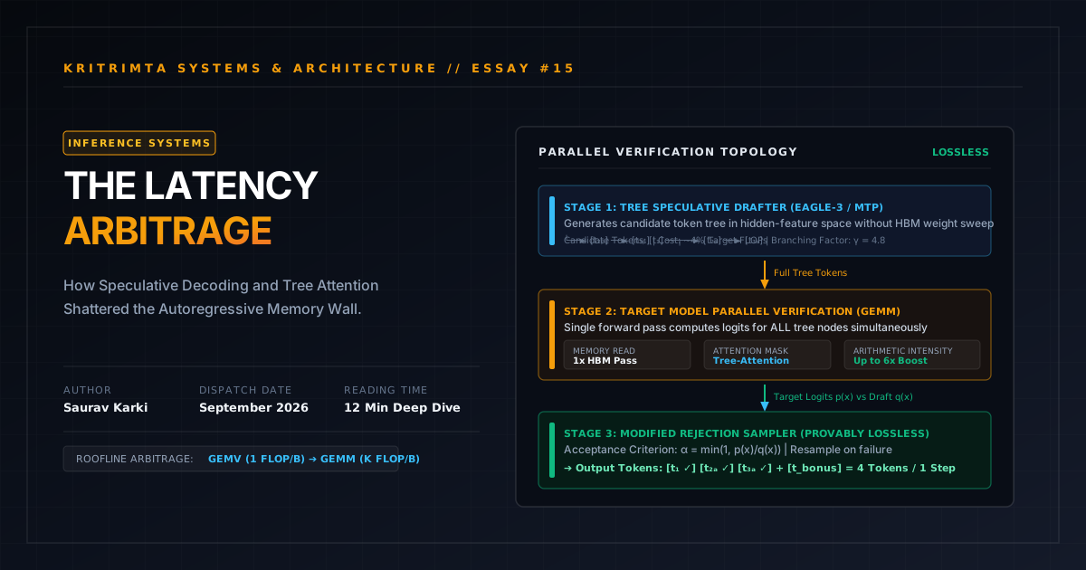
Speculative decoding resolves the memory bandwidth bottleneck by exploiting an asymmetric truth of computation: verifying a sequence of tokens is fundamentally cheaper than generating that sequence token by token.
Instead of invoking the massive 70B target model $K$ times sequentially to generate $K$ tokens—which requires $K$ complete sweeps across 140 GB of HBM—speculative decoding divides the problem into two distinct asynchronous phases:
┌────────────────────────────────────────────────────────────────────────────────┐
│                   THE SPECULATIVE DECODING EXECUTION PIPELINE                  │
├────────────────────────────────────────────────────────────────────────────────┤
│                                                                                │
│  1. SPECULATIVE DRAFTING (Low-Cost / High-Speed)                               │
│     Draft Engine proposes K candidate tokens via small weights / heads:        │
│     Input Tokens ──► [Draft Engine] ──► { x̃₁, x̃₂, x̃₃, x̃₄ }                    │
│                                                                                │
│  2. PARALLEL VERIFICATION (GEMM Compute Arbitrage)                             │
│     Target Model processes all K candidates in a SINGLE forward pass:          │
│     ┌────────────────────────────────────────────────────────────────────────┐ │
│     │ Large Model Target (70B/400B)                                          │ │
│     │ • All K candidate tokens evaluated simultaneously                      │ │
│     │ • Model weights loaded from HBM ONCE                                   │ │
│     │ • Arithmetic Intensity increases by K×: I = K FLOP/Byte                │ │
│     └───────────────────────────────────┬────────────────────────────────────┘ │
│                                         │                                      │
│                                         ▼ Target Logits P(x)                   │
│  3. MODIFIED REJECTION SAMPLING                                                │
│     Deterministic verification matches exact target distribution:              │
│     { x̃₁: ACCEPTED, x̃₂: ACCEPTED, x̃₃: ACCEPTED, x̃₄: REJECTED }                │
│                                                                                │
│  4. RESULT: 3 Verified Tokens + 1 Corrected Token = 4 Tokens in 1 HBM Pass!   │
└────────────────────────────────────────────────────────────────────────────────┘
The Mathematics of Lossless Verification
A common initial skepticism from systems architects unfamiliar with the literature is: Does speculative drafting compromise model quality, introduce hallucinations, or alter perplexity?
The answer is mathematically no. Through the Modified Rejection Sampling algorithm established by Leviathan et al. (2023) and Chen et al. (2023), speculative decoding is provably lossless. The generated token distribution matches the target model’s output distribution down to the precision of the floating-point implementation.
Let $P(x)$ denote the probability distribution of the next token according to the large target model, and let $Q(x)$ denote the probability distribution from the small draft mechanism.
For each candidate token $\tilde{x}_i$ proposed by the draft model, the target model computes the true distribution $P(\tilde{x}i \mid x{<i})$. The token is accepted with probability:
$$\alpha(\tilde{x}_i) = \min\left(1, , \frac{P(\tilde{x}_i)}{Q(\tilde{x}_i)}\right)$$
If a candidate token is accepted, it is appended to the sequence, and the engine moves to evaluate $\tilde{x}_{i+1}$.
If a candidate token $\tilde{x}_i$ is rejected, the speculative chain terminates at that position. The target model rejects $\tilde{x}_i$ and instantly samples a replacement token from a modified residual distribution $P’(x)$:
$$P’(x) = \frac{\max\left(0, , P(x) - Q(x)\right)}{\sum_{y} \max\left(0, , P(y) - Q(y)\right)}$$
The Lossless Proof
The probability of accepting a token under the joint system is:
$$P(\text{accept } x) = Q(x) \cdot \min\left(1, \frac{P(x)}{Q(x)}\right) = \min\left(Q(x), P(x)\right)$$
The probability of rejecting a candidate and sampling $x$ from the residual distribution $P’(x)$ is:
$$P(\text{reject and sample } x) = \left(1 - \sum_y \min(Q(y), P(y))\right) \cdot P’(x)$$
Substituting $P’(x)$:
$$P(\text{reject and sample } x) = \max(0, P(x) - Q(x))$$
Summing both mutually exclusive execution paths:
$$P_{\text{final}}(x) = \min(Q(x), P(x)) + \max(0, P(x) - Q(x)) = P(x)$$
The result is exact: the final output distribution is strictly equal to $P(x)$. The draft model is never allowed to bias the output. It serves strictly as a computational catalyst to unlock parallel verification across the target model’s weights.
3. From Naive Drafting to Tree Attention: The EAGLE-3 Revolution
While the mathematical formulation of speculative decoding was sound in 2023, early implementations suffered from practical systems deficiencies:
- Vocabulary Incompatibility: Independent draft models (e.g., using a 1B model to draft for a 70B model) often utilized mismatched tokenizers or required expensive conversion matrices.
- Sequential Drafting Overhead: If the draft model itself had to execute $K$ autoregressive steps sequentially, the accumulated latency of the drafter eroded the gains of the target verification pass.
- The First-Error Cliff: In linear speculative chains, if the first drafted token $\tilde{x}_1$ was rejected, all subsequent drafted tokens ${\tilde{x}_2, \dots, \tilde{x}_K}$ were discarded immediately, wasting compute.
Linear Speculative Chain (Fragile):
[ t₁ ] ──► [ t₂ (REJECTED) ] ──x   [ t₃ (Wasted) ]   [ t₄ (Wasted) ]
Result: Only 1 token generated; draft overhead wasted.

Tree-Attention Speculative Topology (Robust):
                 ┌──► [ t₂ₐ (ACCEPTED) ] ──► [ t₃ₐ (ACCEPTED) ] ──► [ t₄ₐ ]
[ t₁ (ACCEPTED) ]┤
                 └──► [ t₂ᵦ (Alternative) ] ──► [ t₃ᵦ ]
Result: 3 tokens accepted along Path A despite branching divergence!
EAGLE-3: Feature-Space Drafting
The architectural solution that dominates 2026 inference engines is EAGLE (Extrapolation Algorithm for Greater Language-model Execution), currently in its third generation (EAGLE-3).
EAGLE-3 abandons the naive concept of drafting in token space using a secondary standalone language model. Instead, it attaches an ultra-lightweight transformer layer (often a single attention block) directly to the target model’s upper hidden states.
┌─────────────────────────────────────────────────────────────────────────────┐
│                           EAGLE-3 TOPOLOGY FLOW                             │
├─────────────────────────────────────────────────────────────────────────────┤
│                                                                             │
│   Target Model Top Layer ────► Hidden State Vector (h_t)                    │
│                                           │                                 │
│                                           ▼                                 │
│                           ┌───────────────────────────────┐                 │
│                           │   EAGLE-3 Single-Layer Head   │                 │
│                           │   (Drafts Next Hidden State)  │                 │
│                           └───────────────┬───────────────┘                 │
│                                           │                                 │
│                     ┌─────────────────────┴─────────────────────┐           │
│                     ▼                                           ▼           │
│           Candidate State (h̃_{t+1})                   Candidate State (h̃_{t+2})│
│                     │                                           │           │
│                     ▼                                           ▼           │
│           Target LM Head (Shared)                     Target LM Head (Shared)│
│                     │                                           │           │
│                     ▼                                           ▼           │
│           Draft Token Tree (T) ─────────────────────► Target Verifier       │
│                                                                             │
└─────────────────────────────────────────────────────────────────────────────┘
Rather than sampling discrete tokens and re-embedding them from scratch, EAGLE-3 predicts the sequence of future hidden features ($h_{t+1}, h_{t+2}, \dots$). Because hidden states contain rich contextual representations, feature extrapolation achieves an acceptance rate ($\alpha$) between $82%$ and $91%$ on complex coding and reasoning benchmarks, compared to $55%$–$65%$ for standard small-model drafting.
Tree-Masked Verification
To solve the “First-Error Cliff,” EAGLE-3 constructs a speculative candidate tree rather than a linear sequence.
Using a custom 2D causal attention mask, the target model verifies an entire directed acyclic graph (DAG) of potential token trajectories in a single forward pass:
Tree Attention Mask Matrix:
Token:    Root  L1_A  L2_A1 L2_A2 L1_B  L2_B1
Root   [   1     0     0     0     0     0   ]
L1_A   [   1     1     0     0     0     0   ]  <-- Path A branch
L2_A1  [   1     1     1     0     0     0   ]  <-- Path A1 leaf
L2_A2  [   1     1     0     1     0     0   ]  <-- Path A2 leaf
L1_B   [   1     0     0     0     1     0   ]  <-- Path B branch
L2_B1  [   1     0     0     0     1     1   ]  <-- Path B1 leaf
In this formulation, the target model evaluates tokens along multiple probable trajectories simultaneously. Even if the primary branch diverges at token two, the verifier can accept tokens from an alternative branch, guaranteeing a high mean accepted length ($\tau$).
The expected token yield per verification step follows:
$$\mathbb{E}[\text{Yield}] = 1 + \sum_{k=1}^{K} \prod_{j=1}^{k} \alpha_j$$
With tree attention and acceptance rates exceeding $\alpha = 0.85$, modern serving engines routinely achieve an average yield of 3.8 to 4.5 accepted tokens per target forward pass.
4. Multi-Token Prediction (MTP) and Native Co-Design
While EAGLE-3 provides an external draft harness for frozen models, frontier model architectures in 2026 are increasingly integrating speculative capability natively into their pre-training objectives via Multi-Token Prediction (MTP).
Pioneered in models like DeepSeek-V3 and Meta’s 2025/2026 research clusters, MTP modifies the fundamental loss function of the language model during pre-training:
$$\mathcal{L}{\text{MTP}} = \mathcal{L}{\text{next-token}} + \sum_{k=1}^{M} \lambda_k \mathcal{L}{\text{token}{t+k}}$$
┌─────────────────────────────────────────────────────────────────────────────┐
│                    NATIVE MULTI-TOKEN PREDICTION (MTP)                      │
├─────────────────────────────────────────────────────────────────────────────┤
│                                                                             │
│                     Shared Model Backbone (70B / 671B MoE)                  │
│                     ══════════════════════════════════════                  │
│                                       │                                     │
│               ┌───────────────────────┼───────────────────────┐             │
│               ▼                       ▼                       ▼             │
│      [ Primary Head ]        [ Speculative Head 1 ]  [ Speculative Head 2 ] │
│         Predicts t+1                Predicts t+2            Predicts t+3    │
│                                                                             │
└─────────────────────────────────────────────────────────────────────────────┘
During training, auxiliary shallow heads learn to predict tokens $t+2$ and $t+3$ conditioned on the representations formed by the primary trunk.
During inference, these auxiliary heads function as a zero-memory-overhead draft engine:
- The base model computes token $t+1$.
- Heads 1 and 2 output predictions for $t+2$ and $t+3$ instantaneously via simple linear projections.
- In the subsequent cycle, those candidates are validated in parallel.
MTP eliminates the need to run an auxiliary model or maintain separate KV cache infrastructure for a drafter. The speculative engine is fused directly into the neural architecture.
5. The Concurrency Paradox: When Speculative Decoding Fails
As an engineering publication dedicated to empirical rigor, Kritrimta must state an uncomfortable operational truth: Speculative decoding is not universally beneficial.
Its efficacy is strictly a function of system concurrency and hardware saturation.
       THROUGHPUT VS LATENCY ARBITRAGE ACROSS BATCH SIZES
  Speedup Ratio
      ▲
  4x  │  ████████████  (Batch Size = 1: 3.8x Speedup)
      │  ████████████
  3x  │  ████████████
      │  ████████████  ████████  (Batch Size = 8: 2.4x Speedup)
  2x  │  ████████████  ████████
      │  ████████████  ████████  ██████  (Batch Size = 32: 1.5x Speedup)
  1x  ├──████████████──████████──██████──┬───────────────────────────── Baseline
      │                                  │  ████  (Batch Size = 128: 0.85x Regress)
  0x  └──────────────────────────────────┴───────────────────────────► Batch Size
The Mathematics of Batch Saturation
Speculative decoding exploits surplus compute. At a batch size of $B = 1$, the GPU’s Tensor Cores are $99%$ idle, meaning verifying 5 tokens costs virtually the same wall-clock time as verifying 1 token.
However, consider an enterprise serving cluster operating under heavy concurrency with a batch size of $B = 128$:
- At $B = 128$, the total volume of data passing through the cores scales by $128\times$.
- The arithmetic intensity of standard autoregression naturally shifts from $1.0\text{ FLOP/byte}$ to:
$$I_{\text{batched}} = 128 \times 1.0 = 128\text{ FLOP/Byte}$$
At $128\text{ FLOP/byte}$, the GPU is no longer memory-bandwidth bound. It has crossed the knee of the Roofline curve and reached the compute-bound ceiling.
If you introduce speculative decoding into a compute-saturated system:
- The verification forward pass must now evaluate $128 \times K$ tokens, which requires real, non-trivial FLOP capacity.
- The compute overhead of drafting and tree-mask maintenance begins competing directly with actual output tokens for Tensor Core cycles.
- If the acceptance rate drops (e.g., in highly stochastic sampling tasks), the computational cost of wasted verifications drags net throughput below baseline autoregression.
Production Rule of Thumb
In production runtimes like vLLM and TensorRT-LLM, modern schedulers deploy Dynamic Load-Aware Speculative Scheduling (DLS):
- Interactive Mode ($B \le 16$): Speculative decoding is fully engaged. Latency is minimized, slashing Time-Per-Output-Token (TPOT) by $60%–75%$.
- Saturated Mode ($B \ge 64$): Speculative decoding dynamically disables draft branches or scales $K$ down to 0, pivoting the GPU back to pure batched GEMM throughput.
6. Comprehensive Architectural Comparison
The trajectory of inference acceleration reflects a systematic shift from raw matrix multiplication toward intelligent verification topologies:
| Evaluation Metric | Naive Autoregression | Standalone Small Drafter | Medusa Multiple Heads | EAGLE-3 Feature Tree | Native MTP (DeepSeek-V3) |
|---|---|---|---|---|---|
| Arithmetic Intensity | $\approx 1.0\text{ FLOP/B}$ | $\approx 2.5\text{ FLOP/B}$ | $\approx 3.2\text{ FLOP/B}$ | $\approx 4.8\text{ FLOP/B}$ | $\approx 3.5\text{ FLOP/B}$ |
| Typical Latency Speedup | $1.0\times$ (Baseline) | $1.6\times - 2.1\times$ | $2.2\times - 2.8\times$ | $3.2\times - 4.2\times$ | $2.4\times - 3.1\times$ |
| Acceptance Rate ($\alpha$) | N/A | $55% - 68%$ | $65% - 75%$ | $82% - 91%$ | $70% - 82%$ |
| Draft Overhead | Zero | High (Full forward passes) | Low (Simple MLP heads) | Ultra-Low (Single layer) | Negligible (Fused heads) |
| VRAM Overhead | Baseline | $+15% - 25%$ (2nd model) | $+3% - 5%$ | $+1% - 3%$ | $+2%$ (Pre-trained) |
| Token Verification | Sequential | Linear Chain | Multi-Head Cartesian | 2D Tree Mask Attention | Linear / Shallow Tree |
| Distribution Invariance | Native | Provably Lossless | Provably Lossless | Provably Lossless | Provably Lossless |
| Integration Complexity | Minimal | Medium (Dual engines) | Medium (Extra heads) | Moderate (vLLM / SGLang) | Native / Day-Zero |
7. Production Engineering Implementation
In modern serving engines, deploying speculative decoding requires minimal application-level scaffolding thanks to deep integration within frameworks like vLLM and TensorRT-LLM.
Below is a production-grade configuration deploying an EAGLE-3 speculative tree engine on top of a 70B parameter model using vLLM:
from vllm import LLM, SamplingParams

# Configure Target Model with EAGLE-3 Speculative Acceleration
llm = LLM(
    model="meta-llama/Llama-3.3-70B-Instruct",
    tensor_parallel_size=4,
    speculative_model="yuhuili/EAGLE3-LLaMA3-70B-Instruct",
    num_speculative_tokens=5,             # Maximum speculative tree depth (K)
    speculative_draft_tensor_parallel_size=1, # Drafter runs on single GPU to minimize sync
    use_v2_block_manager=True,            # Optimized PagedAttention for tree KV cache
    enable_chunked_prefill=True,          # Interleaves speculative drafting with prefill
    gpu_memory_utilization=0.90,
)

# Standard sampling parameters: Rejection sampler guarantees exact matching
sampling_params = SamplingParams(
    temperature=0.6,
    top_p=0.9,
    max_tokens=2048,
)

prompts = [
    "Implement an asynchronous lock-free ring buffer in Rust with memory fencing."
]

outputs = llm.generate(prompts, sampling_params)

for output in outputs:
    # Telemetry data shows speculative acceptance efficiency
    print(f"Generated Text: {output.outputs[0].text[:100]}...")
    metrics = output.metrics
    print(f"Speculative Acceptance Rate: {metrics.spec_decode_acceptance_rate:.2%}")
    print(f"Mean Accepted Tokens / Step: {metrics.spec_decode_mean_accepted_tokens:.2f}")
Key Engineering Guardrails
When configuring speculative pipelines in mission-critical environments, production teams must adhere to three non-negotiable architectural practices:
- Tree KV Cache Garbage Collection: Tree-attention produces branching paths where non-selected branches are rejected. Serving engines must implement immediate KV cache pruning (e.g., vLLM’s
v2_block_manager) to reclaim VRAM allocated to discarded candidate leaves. - Tensor Parallelism Disaggregation: Do not run the draft model across the same tensor-parallel (TP) rank split as the target model. If your 70B model runs across 4 GPUs ($TP=4$), running a tiny draft model across $TP=4$ introduces excessive
all-reducecommunication latency that outstrips computation time. Run the drafter on $TP=1$ and broadcast candidate tokens. - Draft Precision Quantization: Draft models and EAGLE heads should always run in FP8 or INT4 precision. Since the target model performs mathematically rigorous rejection sampling, minor numerical discrepancies in the draft phase never affect final output precision—they only cause negligible fluctuations in acceptance probability.
8. Frequently Asked Questions
Does speculative decoding alter the model’s creative or reasoning ability?
No. This is the foundational property of the algorithm. Through modified rejection sampling, speculative decoding is mathematically proven to sample from the exact same probability distribution as the target model. Whether you are generating creative poetry or verifying a complex mathematical proof, the outputs are statistically indistinguishable from native generation.
Can speculative decoding be combined with FP8 and INT4 quantization?
Yes. In fact, speculative decoding and weight quantization are highly synergistic. Quantizing the target model from FP16 to FP8 doubles the bandwidth-limited token generation speed. Layering speculative decoding on top multiplies that speedup by an additional $2.5\times$ to $3.5\times$, delivering aggregate speedups approaching $7\times$ over raw FP16 baselines.
What happens if the prompt requires high temperature (stochastic sampling)?
As sampling temperature ($T$) increases, the target model’s probability distribution flattens, increasing output entropy. This slightly lowers the token acceptance probability $\alpha$, reducing the mean accepted tokens per step from $\sim 4.2$ down to $\sim 2.8$. However, even at elevated temperatures, speculative decoding consistently delivers a net positive speedup over sequential decoding.
Why is speculative decoding especially critical for reasoning models (e.g., DeepSeek-R1, OpenAI o-series)?
Reasoning models allocate massive “test-time compute” to internal deliberation tokens before generating a final answer. A complex prompt can easily trigger 3,000 internal thinking tokens. Under sequential autoregression (30 tokens/sec), a user waits 100 seconds for an answer. Speculative decoding pushes throughput to 120+ tokens/sec, compressing that delay down to under 25 seconds—the difference between an unusable interface and real-time interaction.
The Verdict: The Fallacy of the Von Neumann Token
For more than seven decades, computer architecture has struggled against the Von Neumann bottleneck: the fundamental physical separation between the logic units that process data and the memory buses that store it.
When the deep learning revolution began, we believed we had broken that constraint by packing thousands of parallel execution threads onto monolithic silicon dies. But sequential autoregression stealthily re-introduced the Von Neumann tax in its most insidious form: one token, one memory sweep.
We convinced ourselves that generating language is an inherently sequential cognitive act—that a machine, like a human, must contemplate word $t$ before it can possibly conceive word $t+1$.
It was a failure of systems imagination.
Language generation is only sequential if generation and verification are forced into the same monolithic execution pass. By separating the cheap, high-entropy intuition of drafting from the rigorous, parallel verification of a target model, speculative decoding demonstrates that language generation is massively parallelizable.
In 2026, building inference infrastructure around naive autoregression is computational malpractice. The memory bandwidth wall is real, but it is a wall of our own making.
The future of artificial intelligence does not belong to those who wait for wider memory buses. It belongs to systems architects who exploit the latency arbitrage of parallel verification.
Subscribe to The Kritrimta Dispatch for fortnightly deep dives into AI systems architecture, silicon engineering, and computational economics.